Suddenly Instantaneous
In which I recount how I relearned (learned?) some trigonometry, some calculus, and a few things about floating point numbers. Knowledgeable readers: my deepest apologies.
In brief: In many cases, the frequency of a sound is constant or nearly constant. That is, the frequency does not change over time. In other cases, however, it does change, and when synthesizing sounds with non-constant frequency, you must carefully consider what the frequency is at each moment in time. We need to understand and compute the instantaneous frequency.
Naively…
One foundational part of a software sound synthesizer is generating sine waves. (I’m writing a software synthesizer and therefore need to generate sine waves.) I learned in secondary school that a sine wave is determined by its frequency and initial phase. (I’m ignoring that initial phase, which is important when combining multiple waves, but not perceptible in a single wave and just confuses things here.)
I learned that a wave $s$ with frequency $f$ (in hertz) can be written as function of time as follows:
\[s(t) = \sin(2 \pi f t)\]Where $\sin$ is the ratio between length of the side of a right triangle opposite the given angle and the hypotenuse of that triangle. Right? Right.
While some types of synthesis use sine waves whose frequencies are constant (for example, additive synthesis), others require frequencies that change over time. Examples include implementing a vibrato effect and frequency modulation (FM) synthesis, as well as a frequency “sweep” (where the frequency of a single tone increases over time).
As an algebraically-minded person, I assumed (naively!) that even if the frequency itself varied as a function of time, I could still just substitute $f$ with its definition. For example, if the frequency started at 0 Hz and increased by 500 Hz every second, as in:
\[f(t) = 500t\]Then…
\[s(t) = \sin(2 \pi (500t) t) = \sin(1000 \pi t^2)\]But listening to the waveform generated by this equation, I knew that some things (perhaps many things!) were wrong. Reader, listen:
What are all of those sounds?! That’s a lot more than a single sine wave! And yet the code was nothing more than the equation shown above. I was baffled by how such a simple piece of code could yield such a complex sound.
Here’s what the spectrum looks like as a function of time:
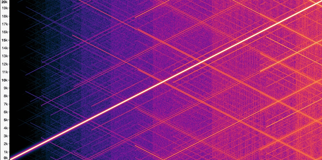
You can see the main tone as the bright diagonal line from the lower left to the upper right. The side tones are all of the other diagonal lines.
Those additional tones were not affected by changing any parameters of the synthesizer (for example, sampling rate, buffer size, output device). The sweep didn’t cross the Nyquist frequency, so they weren’t some sort of aliasing. On the other hand, their slopes would change with the slope of the frequency sweep, and they even occurred when the frequency was constant (though to a lesser extent).
My real clue was that these additional tones always got more numerous and more intense over time; that is, they seemed to be related to some sort of compounding error.
In my sound generation system, I’m treating the inputs and outputs of primitives like $\sin$ uniformly: I’m using the same type for both inputs and outputs. Since the audio library I was using only supported 32-bit floating point numbers, those were also the numbers used for all of the intermediate computation. After 10 seconds, the values passed to the $\sin$ function are greater than $10^6$ and so the precision is only about $10^{-1}$. Errors of that magnitude are remarkably audible!
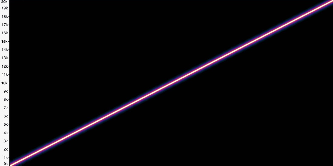
When I changed the code to use 64-bit floating point numbers, this was the result:
This output is much cleaner sounding, and its spectrum looks cleaner too.
But there was still one big problem: if $f(t) = 500t$ why did the tone reach 20 kHz after 20 seconds instead of only 10 kHz? Why was the frequency increasing twice as fast as it should?
Setting the Pace
To explain, let’s take an example from a different domain. Instead of waves and frequency, let’s take position and speed. Say that I have a friend who is a running a race, and I want to meet that friend part way through the race to offer them some water. I know that they plan to run at a speed of 10 miles per hour. That is, their speed is a constant. (In this, er, running example, I’m assuming that $t$ is measured in hours.)
\[v(t) = 10 \text{ miles/hour}\]From this I can calculate where to meet them based on their position at a given time. In addition to some rudimentary trigonometry, I also learned in secondary school that speed is the derivative of position, and therefore position is given by the integral of speed.
\[x(t) = \int_0^t v(\tau) \ d\tau \text{ miles}\]Which is, of course, just…
\[x(t) = \int_0^t 10 \ d\tau = 10 t - 0 t = 10t \text{ miles}\]That is, if I know how many hours have passed, I just multiply that by 10 to find my friend’s location. It will surprise no one that my friend will have run 5 miles after half an hour.
But what if my friend set their initial pace overconfidently? What if, after half an hour they need to slow down to half their initial speed? That is, their speed is now given as:
\[v(t) = \begin{cases} 10 \text{ miles/hour} & \text{for } 0 \le t < 0.5 \\ 5 \text{ miles/hour} & \text{for } 0.5 \le t \end{cases}\]And naively, you might try to calculate their position by integrating their speed in a piecewise manner:
\[x(t) = \begin{cases} 10t \text{ miles} & \text{for } 0 \le t < 0.5 \\ 5t \text{ miles} & \text{for } 0.5 \le t \end{cases}\]But of course even a quick inspection will reveal a problem at $t = 0.5$, where my friend, having run 5 miles in the first half hour, will suddenly (and disappointingly) find themselves transported back to the 2.5 mile mark.
To properly calculate their position after the first half hour, we need to account for their faster pace during that first half hour. That is, we need to add in the $10 \text{ miles/hour} \cdot 0.5 \text{ hours} = 5 \text{ miles}$ that they ran during that first half hour, and then subtract that half hour when determining the contribution of their slower pace.
\[x(t) = \begin{cases} 10t \text{ miles} & \text{for } 0 \le t < 0.5 \\ 5 + 5 \cdot (t - 0.5) \text{ miles} & \text{for } 0.5 \le t \end{cases}\]Not to put too fine a point on it, but my friend’s position at a given time depends not just on their speed a given moment, but on their speed at every moment in time up to that point!
Acutely Angular
Remember that sound is a result of air particles moving back and forth, which cause your ear drums to move back and forth, which eventually stimulate nerves in your inner ear and create the sensation of hearing. And even if a sound wave travels from you to me when you speak, individual air particles don’t move that far: each one just goes back and forth a little bit. This displacement (written here as $s$) is important in sound synthesis, since it’s the displacement of a speaker membrane creates those sound waves, and displacement is roughly what is being measured by individual samples.
Since we’re interested in generating sine waves, we know that displacement as a function of time can be written like this:
\[s(t) = \sin(\phi(t))\]Where $\phi(t)$ is the angular displacement or phase at a given moment in time $t$ and is measured in radians. We’re going to use phase as our analogue to the runner’s position $x(t)$. I find it helpful to visualize phase as the angle of a unit vector rotating counterclockwise around the origin. $\phi$ increases with time, but since we are going to pass it to the $\sin$ function, we can also always take the value of $\phi \hspace{-0.3em} \mod 2 \pi$.
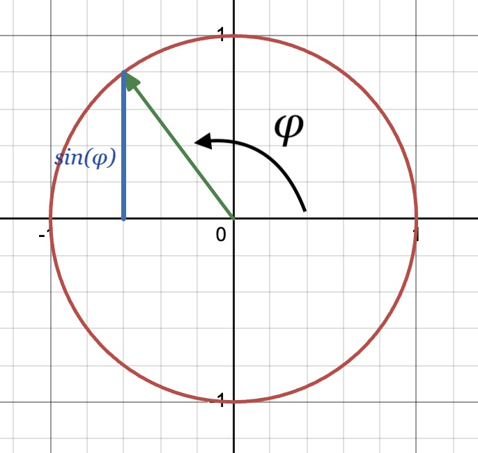
In this context, the sine of $\phi$ is the distance between the x-axis and the end of the unit vector. Or equivalently, it’s the projection of that vector onto the y-axis or the “height” of the vector.
To meet our original goal then, we generate a series of phases, which we will then use to compute a series of displacements such that those displacements will approximate a sine wave with the desired frequency.
Note that the frequency of the sine wave — the rate at which the wave complete a cycle — is the same as the rate at which that vector completes one revolution. This angular frequency $\omega$ is the rate of change of $\phi$ measured in radians/second. (Angular frequency is just a constant times frequency measured in hertz.) That means that angular frequency $\omega$ is analogue of the runner’s speed $v$. Just like we used the runner’s speed to compute position, we’re going to use angular frequency to compute the phase.
One thing that’s nice about angular frequency is that, for constant angular frequency $\omega$, the change of phase $\phi$ for a given duration of time is always the same, regardless of what the initial value of $\phi$ is. This shouldn’t be too surprising, given that “constant angular frequency” is just another way of saying that “phase changes at a constant rate.” That is, if $\omega$ is constant, then we can pick $\Delta t$ to determine some $C$ for which the following holds for any value of $t$.
\[\phi(t) - \phi(t + \Delta t) \text{ mod } 2\pi= C\]This is different from the behavior of $\sin(\phi(t))$, which even at constant frequency has no such equivalent notion of “constant change.” For me, this simple behavior of phase with constant angular frequency makes it a good foundation for thinking about the phase of sine waves with more complex (and time-dependent) angular frequencies.
An aside on perception
As my friend is running, it’s easy for me to perceive where they are at any moment in time, but it’s much more difficult to perceive how fast they are running in that instant. Of course, if I measure their position at two points in time, I can determine their average speed, or if I watch them run for a few seconds, I can tell if they are going fast or slow. But in general, for people and objects as big (and slow) as my friend, position seems to be the primary way I observe them, while speed takes second place.
While sound is fundamentally caused by the displacement of particles air and oscillating changes in air pressure, we don’t perceive those displacements. Instead, the primary way that we perceive sound is its frequency. So while we might start with a runner’s positions over time to determine their speed, if I want my synthesizer to work properly, I need to start with angular frequency and work back to determine phase.
A Phased Approach
Just as we used the integral of speed $v$ to calculate the runner’s position $x$, we can use the integral of angular frequency $\omega$ to calculate the phase $\phi$ (and eventually displacement $s$). That is, like position can be computed by adding up the infinitesimal changes over time (aka speed), phase can also be computed by adding up infinitesimal changes over time (aka angular frequency).
\[\phi(t) = \int_0^t \omega(\tau) \ d\tau\]I now know that:
- (Angular) frequency is one of the the primary observable qualities of sound (as pitch)
- (Angular) displacement can be computed by integrating the (angular) frequency
We can now properly compute the samples (that is, the displacements) for a frequency sweep determined by:
\[f(t) = 500t\]Or equivalently as angular frequency:
\[\omega(t) = 2\pi \cdot f(t) = 1000\pi t\]If we assume that the initial phase is zero, we substitute and use the power rule:
\[\phi(t) = \int_0^t \omega(\tau) \ d\tau = \int_0^t 1000\pi \tau \ d\tau = \frac{1}{2} 1000 \pi t^2 = 500 \pi t^2\]Which is exactly a factor of two off from the definition I erroneously derived above! That’s why my naive sweep ended at 20 kHz instead of 10 kHz. As when integrating the speed of my friend the running, it’s important to understand the frequency at each point in time, the instantaneous frequency. If we assume that the frequency has been 5 kHz the entire time, then we’ll compute the phase at the 10 second mark incorrectly (analogous to when we assumed that the runner had been running at 5 miles/hour the entire race). Just as when using velocity to compute position, we must consider the frequency at each point up to $t$ to compute the displacement at time $t$.
Incidentally, there’s nothing wrong with equation for sine waves that I learned in secondary school, it’s just that if the frequency is constant, then the integral is trivial:
\[\phi(t) = \int_0^t 2\pi \cdot f \ d\tau = 2\pi \cdot f \cdot \int_0^t 1 \ d\tau = 2\pi \cdot f \cdot t\]Routinely Rectangular
My synthesizer differs from this example in two ways:
- It’s based on samples: it only needs to compute the phase at discrete moments in time.
- It supports frequencies that vary in arbitrary ways, including from input devices, and can’t use an analytic solution to the integral.
Happily, these come together to support a simple and accurate implementation. Indexing at discrete moments in time $t_n$ and using square brackets as in $\phi_\text{approx}[t_n]$ to represent discrete-time phase, we can approximate phase as:
\[\phi_\text{approx}[t_n] = \sum_{i=0}^n \omega(t_i) \Delta t = \sum_{i=0}^n \frac{\omega(t_i)}{f_s}\]Where $\Delta t$ is the length of time represented by one sample and $f_s$ is the sampling rate (and $\Delta t = 1/f_s$). Put another way, this equation says if we divide the change-in-phase per second by the number of samples per second, we get the change-in-phase per sample.
Since we care about each of the intermediate values, we can also think of this as the following recurrence:
\[\phi_\text{approx}[t_0] = 0 \\[0.5em] \phi_\text{approx}[t_n] = \phi_\text{approx}[t_{n-1}] + \frac{\omega(t_n)}{f_s} \enspace \text{ (for $n$ = 1, 2, ...)}\]This is efficient (it requires only a few operations per iteration) and doesn’t require a closed-form definition of frequency. Even using only 32-bit floating point numbers, we get a result that sounds and looks good:
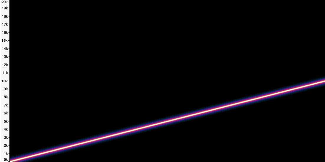
Hooray! Part of the reason that this works well is that, because we’re going to pass $\phi_\text{approx}[t_n]$ to the sine function, we can bound $\phi_\text{approx}[t_n]$ by taking the remainder after dividing it by $2\pi$ at each step:
\[\phi_\text{approx}[t_n] = \left( \phi_\text{approx}[t_{n-1}] + \frac{\omega(t_n)}{f_s} \right) \hspace{-1em} \mod 2 \pi\]And because $\omega(t_n)/f_s$ doesn’t get large either, 32 bits is more than enough precision.
Checking our work
Since we can integrate $\omega(t)$ analytically in the case of a sweep, we can check these discrete approximations by comparing $\phi_\text{approx}[t_n]$ against $\phi(t_n)$. I set up a simple test to check that the approximation is a reasonable match for the exact value. (Here, we still have $\omega(t) = 1000\pi t$, and I’m using $f_s = 100$.)
| $n$ | $t_n$ | $\omega(t_n)$ | $\phi(t_n)$ | $\phi_\text{approx}[t_n]$ | $\epsilon_\phi = \phi_\text{approx}[t_n] - \phi(t_n)$ |
|---|---|---|---|---|---|
| 0 | 0.00 | 0.0 | 0.0000 | 0.0000 | 0.0000 |
| 1 | 0.01 | 31.4 | 0.1571 | 0.3142 | 0.1571 |
| 2 | 0.02 | 62.8 | 0.6283 | 0.9425 | 0.3142 |
| 3 | 0.03 | 94.2 | 1.4137 | 1.8850 | 0.4712 |
| 4 | 0.04 | 125.7 | 2.5133 | 3.1416 | 0.6283 |
| 5 | 0.05 | 157.1 | 3.9270 | 4.7124 | 0.7854 |
| 6 | 0.06 | 188.5 | 5.6549 | 6.5973 | 0.9425 |
| 7 | 0.07 | 219.9 | 7.6969 | 8.7965 | 1.0996 |
| 8 | 0.08 | 251.3 | 10.053 | 11.309 | 1.2566 |
| 9 | 0.09 | 282.7 | 12.723 | 14.137 | 1.4137 |
Whoa… maybe not as accurate as I’d hoped. What’s going on here? Not only is there considerable error, it seems to be getting worse over time.
It’s useful to consider the area-under-the-curve interpretation of the integral for a moment: taking the integral of $\omega$ is the equivalent of measuring the area beneath the line defined by $\omega$. With $\phi_\text{approx}$ we are approximating this by measuring the area of a series of rectangles: multiplying the value of $\omega(t)$ (the height) by $\Delta t$ (the width). Here’s a simple example using the line $y = x$:
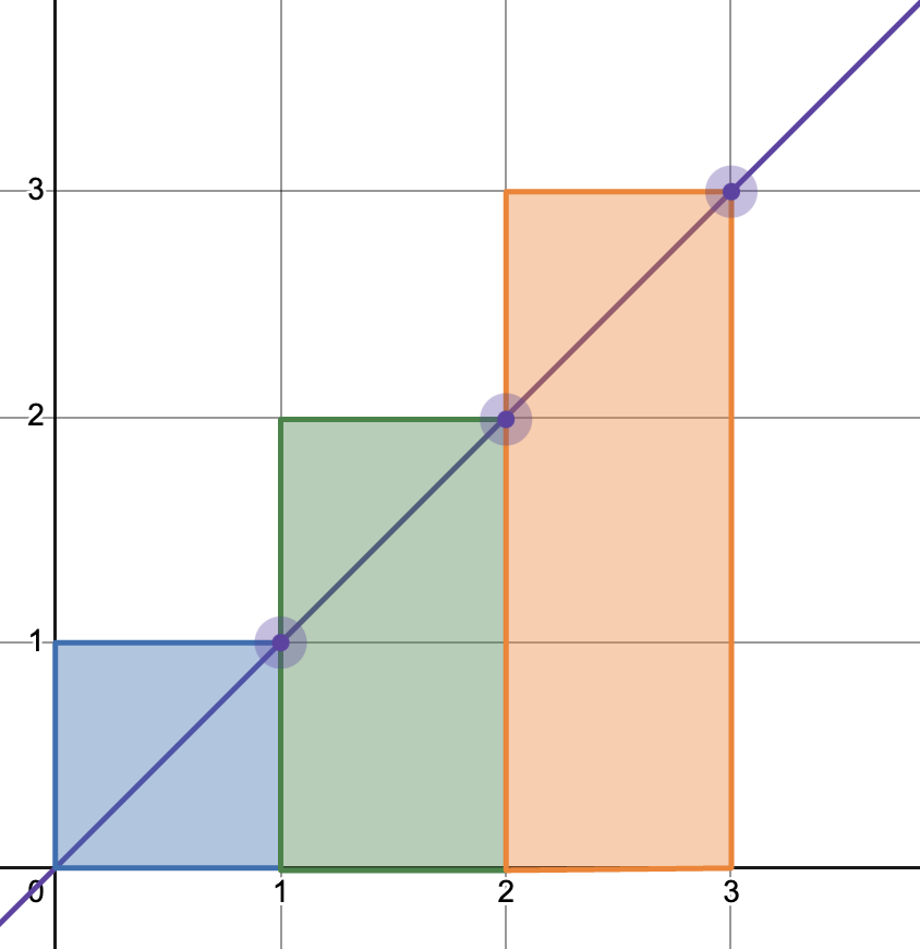
Notice that with the method, the shaded area almost always extends above the line: that is, the sum of the areas of the rectangles is always greater than the area under the line. This will continually overestimate the integral of $y = x$.
A slightly more sophisticated technique is to use two points on the line instead of just one to approximate the area. That is, we use the average of the current and previous points on the line. This is called a trapezoid approximation, since it calculates the area using a series of trapezoids. Here’s the equivalent picture:
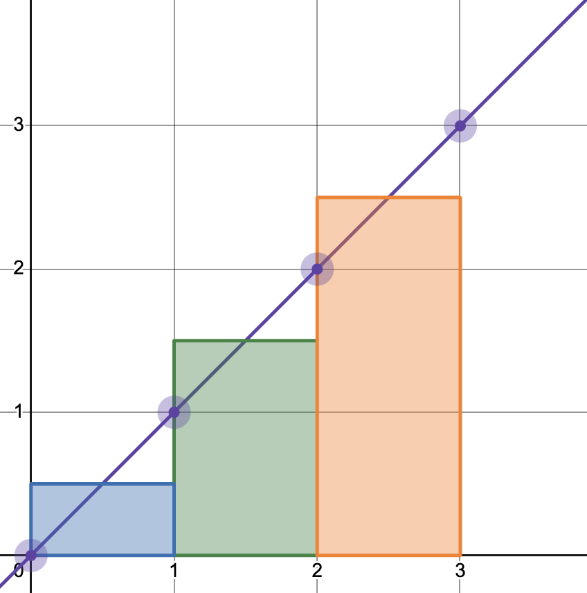
This approximation works much better for linear functions like $y = x$ and $\omega(t) = 1000\pi t$, and in fact the errors in those cases are zero. But why then does the sample above sound reasonable? Why don’t we hear some distortion? There are two answers:
-
The error in associated with a rectangular approximation of a linear frequency sweep leads to only a constant change in the frequency.
-
The test I described and the table above use a ridiculously low sampling rate ($f_s = 100$), which is much lower than the sampling rate used for the audio file ($f_s = 44100$).
Let’s take each of these in turn.
Constantly constant
We took the integral of frequency to determine the phase over time (or rather, we approximated that integral) so we can reverse the process to understand what the true frequency of that series of phases should sound like. That is, we can take the derivative of the the approximation and compare that with the desired frequency $\omega(t)$ to learn how far off the approximation should sound. To do so, we first need to define the approximation at all points in time, not just at the sampled points $t_n$. For some $t$ between $t_{n-1}$ and $t_n$, we will connect those points with a straight line:
\[\phi_\text{approx}(t) = \phi_\text{approx}[t_{n-1}] + \frac{\phi_\text{approx}[t_n] - \phi_\text{approx}[t_{n-1}]}{\Delta t} (t - t_{n-1})\](This is a reasonable thing to do since digital-analog converters will do some smoothing and since a physical speaker membrane can’t instantaneously jump from one position to the next.)
We can substitute the definition of $\phi_\text{approx}[t_n]$ to get:
\[\phi_\text{approx}(t) = \phi_\text{approx}[t_{n-1}] + \frac{\omega(t_n)\Delta t}{\Delta t} (t - t_{n-1}) \\[1em] = \phi_\text{approx}[t_{n-1}] + \omega(t_n) (t - t_{n-1})\]The slope of that segment is exactly $\omega(t_n)$, so the derivative with respect to $t$ is simply:
\[\omega_\text{approx}(t) = \frac{d \phi_\text{approx}(t)}{dt} = \omega(t_n)\]So, again remembering that $t$ is between $t_{n-1}$ and $t_n$, the error in the frequency at time $t$ is:
\[\epsilon_\omega(t) = \omega_\text{approx}(t) - \omega(t) = \omega(t_n) - \omega(t)\]In other words, the error in frequency at time $t$ is given by the difference between the frequency at the time of the next sample after $t$ and the frequency at $t$. Since in this case $\omega(t) = 1000\pi t$ and the difference between $t_n$ and $t$ is at most $\Delta t$, we can bound the error in frequency as a follows:
\[\epsilon_\omega(t) = 1000\pi t_n - 1000\pi t = 1000\pi (t_n - t) < 1000\pi \Delta t\]That is, the error in angular frequency is bounded by a small constant! While the approximated phase is getting farther and farther from the true phase, it’s getting farther at a constant rate, which means that the frequency of the approximation is only shifted by a constant. It still is generating a linear sweep, just one that starts and ends slightly higher than it should. How much higher? The example above uses a sampling rate $f_s$ of 44,100 Hz. This means at any given time, the frequency of the sweep is within than 0.0114 Hz of where it should be.
This is extremely difficult to perceive, not only because the frequency is shifted by such a small amount, but because the frequency of the sweep is changing fast enough to make it hard to compare with any reference tone.
Rates are (damned) high enough
In the example above, the errors incurred by the rectangular approximation weren’t perceptible, so I spent some time looking for cases where they could be heard, and especially for cases where the amount of frequency drift increased over time.
In the linear sweep example above, we can put a tight bound on the error in part because $\omega(t)$ is linear. I suspected that a higher-order function might incur more error, so I started looking at other ways of bounding the error for an arbitrary (differentiable) function. One way to do that is to take the first-order Taylor series approximation of $\omega(t)$, using a nearby point and the derivative of the frequency $\omega’(t_n)$ at that point (and continuing to assume that $t_{n-1} < t < t_n$).
\[\omega(t) \approx \omega(t_n) - \omega'(t_n)(t_n - t) = \omega(t_n) + \omega'(t_n)(t - t_n)\]Put another way, we can approximate the frequency at an arbitrary point, using the frequency at one of the sampled points and the change in frequency at that point.
Plugging this into the definition of the frequency error gives us:
\[\epsilon_\omega(t) \approx \omega(t_n) + \omega'(t_n)(t - t_n) - \omega(t_n) = \omega'(t_n)(t - t_n) < |\omega'(t_n)|\Delta t\]That is, the error is bounded, approximately, by the derivative of the frequency times the distance between samples. Or equivalently,
\[\epsilon_\omega(t) \lessapprox \frac{|\omega'(t_n)|}{f_s}\]If we’re looking for a perceptible error — say, greater than 1 Hz — then the ratio of the angular frequency to the sampling rate would need to be greater than $2\pi$.
\[2\pi < \frac{|\omega'(t_n)|}{f_s}\]That means that for the error to be perceptible, the frequency must change faster than the sampling rate:
\[f_s < |f'(t_n)|\]That’s really fast! The range of human hearing is about 20 Hz to 20,000 Hz, so if $f_s$ = 44,100, the frequency would need to cross that entire range in less than half a second! That’s going to sound like a laser blast, and there’s no way that a 1 Hz shift in frequency is going to be something you can hear.
You might consider a case where the frequency changes quickly, but goes up and down (and therefore stays within the range of human hearing for longer than half a second). But while rectangle method overestimates the integral for increasing functions, it underestimates the integral for decreasing functions, so any errors incurred while going up will be canceled out coming down.
So it turns out that this simple approximation using rectangles is more than good enough: we don’t even need to use the trapezoid method. My intuition for this is that the rectangle method is able to “catch up” with any changes in the frequency at each sample; so unless there are significant changes to the frequency “between” samples, the errors will be small.
Summary
Unlike many other aspects of the physical world, we perceive sound as the derivative of a physical process rather than the process itself: we perceive the frequency of a tone, rather than the displacement of air particles. To faithfully generate sounds with particular frequencies, we must calculate this displacement using the desired instantaneous frequency. This means calculating the definite integral of frequency.
In cases were we can’t (or don’t want to) integrate frequency analytically, we can approximate it using a number of different methods, but for sound generation, a simple rectangular method is sufficient.
While implementing a software synthesizer, I often came across this technique described as “direct digital synthesis.” (Or more specifically, the numerically controlled oscillator portion of DDS.) It seemed to be discussed either in the context of specialized hardware or further software optimizations (for example, using lookup tables to avoid computing $\sin$ for each iteration). Ultimately, however, if we want to synthesize a sine wave with a non-constant frequency — and we can’t compute that integral analytically — we need to do some sort of approximation of that integral. That is, we need to compute a series of discrete sums, and that is exactly what DDS does.
(A final caveat: I’m no expert in these techniques and am simply writing up what I think I’ve learned. It’s possible I’ve made (still more) mistakes! If I have, please let me know.)